Methods of Curve Setting: Four methods are commonly used by using tape or chain together with an equipment:
1) Offsets from Long Chord, Method: From Fig 

EF and EQ1 are the offsets at the mid-point E.

Let Q be a point be taken at the curve AFC between the point A and F.

Now PQ = Ox and PE = x. Draw QQ1 parallel to AE meeting the line EF at Q1.

Draw OQ cutting the line AE at point P and meeting the curve AFC at point Q.

From  OQQ1: (OQ)2 = (QQ1)2 + (OQ1)2 …………. (i) [  OQ1Q = 90o ]

OQ = R and QQ1 = x OQ1 = OE + EQ1 = (R – QO) + Qx [OE = R – QO]

From
[(R – QO) + Qx] = R2 – x2

QO = EF = OF – OE = R – R2 – (L/2)2 [OF = R; and OE = R2 – (L/2)2]
OE = R2 – (L/2)2 How? (OA)2 = (AE)2 + (OE)2  (OE)2 = (OA)2 - (AE)2

Similarly Qx = R2 – x2 – [ R – (R – R2 – (L/2)2)] = R2 – x2 – R2 – (L/22)

Successive Bisection of Chords or Arcs, Method

: Consider the Fig. 2, join A and C so that it bisects the radius-line OF at point E. Set offset
EF = R [1 - Cos I/2] and EF is the offset at the mid-point E.
Set the offset EF = R [1 – Cos(I/2)] to fix point F on the curve. FA and FC are joined, usually in form of a curve. Bisect them at point Q and Q2 as shown in Fig. 2. Set out the offset PQ and KQ2 each one equal to R [1 – Cos(I/4)] and thus the two points Q and Q2 are fixed on the curve AFC. Join the points AQ, QF, FQ2 and Q2C, and set offsets at their centres equal to R [1 – Cos(I/8)]. Repeat this process and set out the required points to establish the curve.

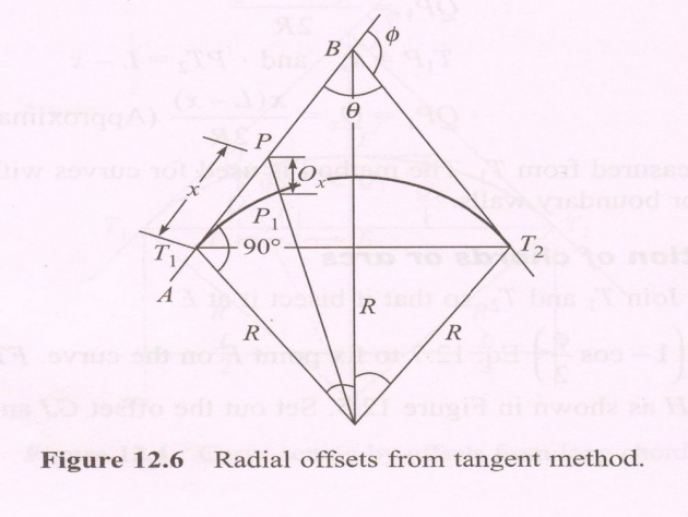
3) Offset from Tangents, Method: Offset is either Radial or Perpendicular to the Tangent.
When the Offset is Radial: Let PP1 = Ox [Refer to Fig. 12.6]
From OPT1, let (OP)2 be equal to (PT1)2 + (OT1)2 [OP = OP1 + PP1]
Or (OP1 + PP1)2 = x2 + R2 Or (R + Ox)2 = x2 + R2 Or R + Ox = x2 + R2
___________________________
Ox = x2 + R2 - R …… (i) An approximate formula related to that given in eq. (i) can be obtained from Binomial Theorem:
_________________________

x2 + R2 = R[1+(x/R)]1/2 = R [1 + 1 x2 + ….. + …. ] = R [1 + 1 x2]
--------------------- -------------------- ------------------------- --------------------------
2 R2 2 R2
So Ox = R [1 + 1 x2] – R  Ox = x2 ……… (ii)

------------------ -------------- ----------------
2 R2 2R
Alternatively from the Properties of Circle, we get:
(Length of Tangent to Offset)2 = PP1(PP1 + 2R) Or (PT1)2 = Ox(Ox + 2R)
x2 = Ox2 + 2ROx As Ox is too small as compared to 2R, so Ox2 can be neglected.  x2 = 2ROx  Ox = x2 / 2R.  It is an approx. formula of calculating the Radial Offset Distance Ox.
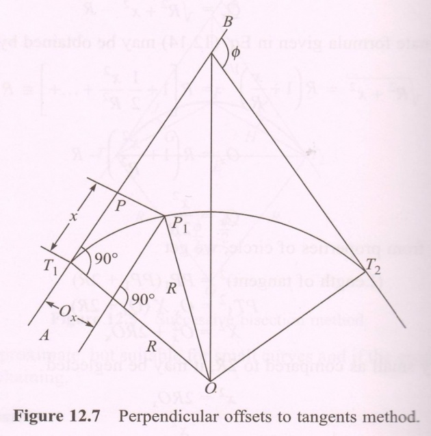
(b) When the Offset is Perpendicular to the Tangent: Let PP1 = Ox perp. To PT1 at T1 drawn along AB. Draw P1P2 parallel to BT1 meeting OT1 at P2 (Fig. 12.7)
__________________________
Now P1P2 = PT1 = x and T1P2 = PP1 = Ox  T1P2 = OT1 - OP2 = R - R2 - x2OT1 = Ox + OP2 = Ox + (OP1)2 - (P1P2)2 = R2 - x2 And Ox = R - R2 - x2
Approx formula can be obtained like the previous case. From eq. (ii) (given on previous slide), we have: We have another formula driven Binomially: Ox = x2 + x4 ……… (iii). This equation represents a parabola, not a
2R 8R3 circle. However, if the Ver.Sin of the curve is less than 1/8th of its chord in the value, then the error is not a big in value

4) Offset from the Chord produced, Method: This method is useful for the long curves in highway (and railway too) when an equipment is not available. This method is fairly accurate than the previous method (Method No. 3). This method can be used even the tangent points T1 and T2 are inaccessible. This method is based on an assumption that for small chords, the chord length is equal to the arc length.

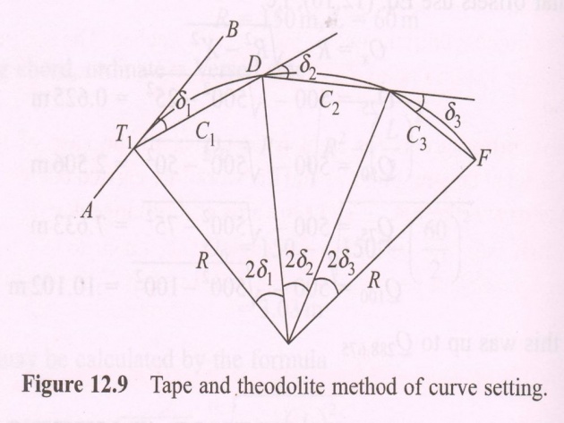
In Fig.  T1 is the first tangent point. D, E, F, etc. are the successive points. C1, C2, C3, etc are the equal chords (lengths of the chords) of T1D, DE and EF. Angle BT1D = 1 Rad (i.e. angle in Radians, denoted as “Rad”) which is equivalent to the angle between tangent BT1 and first chord length T1D.
First Offset O1 ≈ Arc DB  O1 = (T1D)2/2R = C12/2R where C1 is the length of first sub-chord T1D. To obtain the second Offset O2, draw tangent CDD1 to the curve at point D and cut the rear tangent at C. Join T1D and prolong the chord T1D to a point D2 such that DD2 = DE = C2 = Length of the second chord

C

Rankin’s Tangential Angles or Deflection Angle Method

– Tape and Equipment Method: In this method, a tape for measurement of linear distances and an equipment for measuring the angles are used. This method is quite accurate and used to set out the curves of highways and railways. Consider the Fig. 12.9; let T1 be the first tangent point and D, E, F, etc are the successive points on the curve. R is the radius of the curve. C1, C2, C3, etc are the lengths of the chords T1D, DE, EF, etc. 1, 2, 3, etc are the total tangential or deflection angles which the chords T1D, DE, EF, etc make with the first tangent AB. Now chord T1D ≈ C1 BT1D = 1 = ½(T1OD) [As angle T1OD = 21]
ArcT1D/RadiusOT1 =  T1OD.Rad C1 / R = 21 Rad  1 = C1 / 2R Rad

1 = [C1 x 180 x 60] min = 1718.87C1
-------------------- -------------------------- ----------------------------------------------------------------------
2R  R
2 = 1718.87C2 / R 3 = 1718.87C3 / R x = 1718.87Cx / R
Total Tangential (or Deflection) Angle for the first chord T1D = 1  1 = 1
Total Tangential Angle for second chord DE = BT1E = BT1D + DT1E. But from geometry, angle between the tangent and a chord equals the angle which the chord subtends in the opposite segment. Now DT1E is the angle subtended by the chord DE in the opposite segment. Therefor, it is equal to the tangential angle 2 formed between the tangent at D and chord DE.= 1 + 2

Transition Curve: It is also known as Easement Curve. It is a type of Horizontal Curve of varying radius set out between a straight path and circular curve. At the straight path, the radius is infinity. On the other end of the circular curve, transition curve is again provided between the said circular curve until the path becomes straight again. Radius of the Transition Curve is greater than that of circular but smaller than infinity. Transition Curves are essentially provided in the fast moving transportation paths e.g. e.g. Express Highway / Super-highway, Motorway, High Speed .
As soon a vehicle starts undertaking a curve from the straight path, then it starts undergoing the action of Centrifugal Force which tends to throw that vehicle away and overturn. It causes great discomfort to the passengers and likelihood of overturning of the vehicle. In order to balance that Centrifugal Force, outer edge of the path is raised. This procedure of raising the outer edge of the path is known as Banking or Super-elevation or Cant – usually Super-elevation. Amount of Super-elevation to be provided is dependent upon the speed of the vehicle and radius of the curve. In case of Railways, this elevation cannot exceed 15 cm.
The effect of Centrifugal Force can be reduced by increasing the Super-elevation gradually by introducing the Transition Curve between the straight path and circular curve. The second Transition Curve gradually reduced the Super-elevation to zero just at or before the beginning of straight path.