Question_01:Run the Program P1_8 for M = 2 to generate the output signal with x[n] = s1[n] + s2[n] as the input. Whichcomponent of the input x[n] is suppressed by the discrete-time system simulated by this program
Program:
m=2;
n=1:100;
s1=cos(2*pi*.05*n);
s2=cos(2*pi*.47*n);
x=s1+s2;
num=ones(1,m);
y=filter(num,1,x)/m;
subplot(2,2,1);
plot(n,s1);
axis([0, 100, -2, 2]);
xlabel('Time index n'); ylabel('Amplitude');
title('Signal # 1');
subplot(2,2,2);
plot(n,s2);
axis([0, 100, -2, 2]);
xlabel('Time index n'); ylabel('Amplitude');
title('Signal # 2');
subplot(2,2,3);
plot(n,x);
axis([0, 100, -2, 2]);
xlabel('Time index n'); ylabel('Amplitude');
title('Input Signal');
subplot(2,2,4);
plot(n,y);
axis([0, 100, -2, 2]);
xlabel('Time index n'); ylabel('Amplitude');
title('Output Signal');
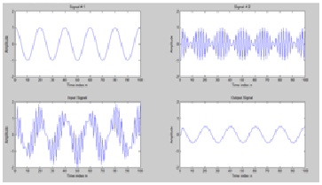
Conclusion
Moving average filter is used to remove signal of high frequency (act as low pass) by decreasing the order of filter(M) we infact compress the signal of high frequency,S2 is compressed.
Qn0_2
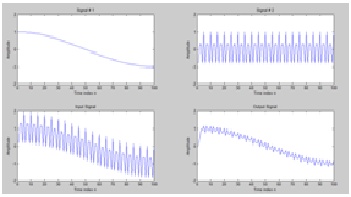
If the LTI system is changed from y[n] = 0.5(x[n] + x[n - 1]) to y[n] = 0.5(x[n] - x[n - 1]), what would be its effect on the input x[n] = s1[n] + s2[n]?
Program:
y[n] = 0.5(x[n] + x[n - 1])
the graph is
If Y[n]=0.5(x[n] - x[n - 1])
Then graph is
The graph show that if we change y[n] then x=s1+s2 after passing through filter will enrich with high frequency signal comparatly
Qn0_3
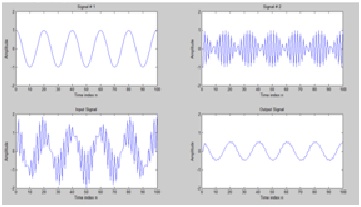
Run Program P1_8 for other values of filter length M, and various values of the frequencies of the sinusoidal signals s1[n] and s2[n]. Comment on your results.
ANSWER:
If we increase the order of filter means we increase the value of ‘m’ then their wil be compression of signal having high frequency and we get signal having low freguency.
By changing frequencing there is no change in magnitude of output signal the output and input signal is compress or expand by increasing and decreasing the freguency of input signal
Qn0_4
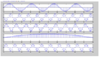
Use sinusoidal signals with different frequencies as the input signals and compute the output signal for each input. How do the output signals depend on the frequencies of the input signal?
M file
function[y]=sinfun(n , f)
y=sin(2*pi*f*n);
end
in command window
n=0:100;
for i=1:5,
f=input('enter frequency');
y=sinfun(n,f);
subplot(5,1,i);
stem(n,y);
end
enter frequency.04
enter frequency .9
enter frequency .09
enter frequency .005
enter frequency .1
Qn0_5
Run Program P1_3 and compare y[n] obtained with weighted input with yt[n] obtained by combining the two outputs y1[n] and y2[n] with the same weights. Are these two sequences equal? Is this system linear?
>> n = 0:40;
a = 2;b = -3;
x1 = cos(2*pi*0.1*n);
x2 = cos(2*pi*0.4*n);
x = a*x1 + b*x2;
num = [2.2403 2.4908 2.2403];
den = [1 -0.4 0.75];
ic = [0 0]; % Set zero initial conditions
y1 = filter(num,den,x1,ic); % Compute the output y1[n]
y2 = filter(num,den,x2,ic); % Compute the output y2[n]
y = filter(num,den,x,ic); % Compute the output y[n]
yt = a*y1 + b*y2;
d=y-yt;
if(yt==y)
disp('they are equal ')
else
disp('they are not equal')
end
subplot(3,1,1)
stem(n,y);
ylabel('Amplitude');
title('Output Due to Weighted Input: a \cdot+ x_{1}+[n]+ b \cdot+ x_{2}+[n]');
subplot(3,1,2)
stem(n,yt);
ylabel('Amplitude');
title('Weighted Output: a \cdot+ y_{1}+[n] + b \cdot+y_{2}+[n]');
subplot(3,1,3)
stem(n,d);
xlabel('Time index n'); ylabel('Amplitude');
title('Difference Signa
they are not equal
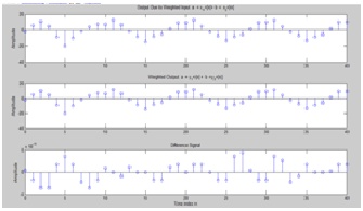
conclusion:
they are almost equal but not exactly this system is linear
as graph show
Qn0_6
Consider another system described by: y[n] = x[n] x[n − 1].Modify Program P1_3 to compute the output sequences y1[n], y2[n], and y[n] of the above system. Compare y[n] with yt[n]. Are these two sequences equal? Is this system linear?
n = 0:40;
a = 2;b = -3;
x1 = cos(2*pi*0.1*n);
x2 = cos(2*pi*0.4*n);
x = a*x1 + b*x2;
num = [1 1];
den = [1];
ic = [0]; % Set zero initial conditions
y1 = filter(num,den,x1,ic); % Compute the output y1[n]
y2 = filter(num,den,x2,ic); % Compute the output y2[n]
y = filter(num,den,x,ic); % Compute the output y[n]
yt = a*y1 + b*y2;
d=y-yt;
if(yt==y)
disp('they are equal ')
else
disp('they are not equal')
end
subplot(3,1,1)
stem(n,y);
ylabel('Amplitude');
title('Output Due to Weighted Input: a \cdot+ x_{1}[n]+ b \cdot+ x_{2}[n]');
subplot(3,1,2)
stem(n,yt);
ylabel('Amplitude');
title('Weighted Output: a \cdot+ y_{1}[n] + b \cdot+y_{2}[n]');
subplot(3,1,3)
stem(n,d);
xlabel('Time index n'); ylabel('Amplitude');
title('Difference Signal')
àthey are not equal
Couclusion:
they are almost equal and they are linear as shown in graph
Qn0_7
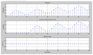
Run Program P1_4 and compare the output sequences y[n] and yd[n - 10]. What is the relation between these two sequences? Is this system time-invariant?
n = 0:40; D = 10;a = 3.0;b = -2;
x = a*cos(2*pi*0.1*n) + b*cos(2*pi*0.4*n);
xd = [zeros(1,D) x];
num = [2.2403 2.4908 2.2403];
den = [1 -0.4 0.75];
ic = [0 0];% Set initial conditions
% Compute the output y[n]
y = filter(num,den,x,ic);
% Compute the output yd[n]
yd = filter(num,den,xd,ic);
% Compute the difference output d[n]
d=y- yd(1+D:41+D);
if(d==0)
disp('they are equal ')
else
disp('they are not equal')
end
% Plot the outputs
subplot(3,1,1)
stem(n,y);
ylabel('Amplitude');
title('Output y[n]');grid;
subplot(3,1,2)
stem(n,yd(1:41));
ylabel('Amplitude');
title(['Output Due to Delayed Input x[n ', num2str(D),']']);grid;
subplot(3,1,3)
stem(n,d);
xlabel('Time index n'); ylabel('Amplitude');
title('Difference Signal');grid;
àthey are equal
Conclusion:
They are exactly equal with yd is shifted version of y by 10th times and they are time invarient
Qn0_8
Consider another system described byY[n]=nx[n]+x[n-1]Modify Program P1_4 to simulate the above system and determine whether this system is time-invariant or not.
n = 0:40; D = 10;a = 3.0;b = -2;
x = a*cos(2*pi*0.1*n) + b*cos(2*pi*0.4*n);
xd = [zeros(1,D) x];
num = [n 1];
den = [1];
ic = 0*[0:40];% Set initial conditions
% Compute the output y[n]
y = filter(num,den,x,ic);
% Compute the output yd[n]
yd = filter(num,den,xd,ic);
% Compute the difference output d[n]
d=y- yd(1+D:41+D);
if(d==0)
disp('they are equal ')
else
disp('they are not equal')
end
% Plot the outputs
subplot(3,1,1)
stem(n,y);
ylabel('Amplitude');
title('Output y[n]');grid;
subplot(3,1,2)
stem(n,yd(1:41));
ylabel('Amplitude');
title(['Output Due to Delayed Input x[n ', num2str(D),']']);grid;
subplot(3,1,3)
stem(n,d);
xlabel('Time index n'); ylabel('Amplitude');
title('Difference Signal');grid;
they are equal
Conclution:
This system is time in varient as shown by graph