1. Objective
The objective of this lab is to introduce you to the classifications of signals and how these classes
of signals can be implemented in MATLAB.
2. Resources Required
• A computer
• MATLAB 7.0 or higher
3. Introduction
Signals are the pattern of variation that contains some sort of information. Information may be
stored in memory or just transient information in real time as in communication systems.
There can be many classifications of signals; some of the classifications are listed below:
1. Continuous Time vs. Discrete Time Signals
2. Analog vs. Digital Signals
3. Periodic vs. Aperiodic Signals
4. Even vs. Odd Signals
5. Deterministic vs. Random Signals
6. Energy vs. Power Signals
3.1 Continuous Time vs. Discrete Time Signals
a) Continuous Time Signals:
Continuous Time Signal is the one whose domain is uncountable, we don’t care about range.
For storing the continuous time signal you need infinite memory which is not possible in any real
system. So, finite no of samples of a continuous time signals are stored. For plotting the
continuous time signals we use plot command, which simply connects the values of intermediate
samples, gives us the illusion of continuous time signals.
In MATLAB we can plot any continuous time signal for example using plot
command as follows:
%Continuous Time Signal Example
A=2; %Amplitude
f=2; %Frequence
phase=pi; %Phase
t=(0:0.01:2*pi)/pi; %Horizontal time axis
plot(t,A*sin(2*pi*f*t+phase));
title('Example of Continuous Time Signal');
xlabel ('Time (pi Units)');
ylabel ('Amplitude');
b) Discrete Time Signals:
Discrete Time Signals are those signals which are purely based upon domain, whose domain is
countable. We don’t care about range of the signal.
In MATLAB we can plot any discrete time signal for example using stem
command as follows:
%Discrete Time Signal Example
A=1; %Amplitude
f=1; %Frequence
phase=pi; %Phase
n=0:10; %Sample Number
stem(n,A*sin(f*n+phase));
title('Example of Discrete Time Signal');
xlabel ('n (Sample Number)');
ylabel ('Amplitude');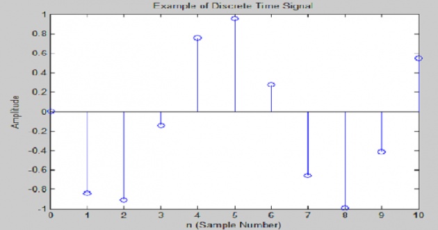
3.2 Analog vs. Digital Signal:
This classification of signal is purely based on range, we don’t care about the domain.
a) Analog Signals:
Analog Signals can take infinite values in range. In MATLAB we can plot any continuous time
signal for example. using plot command as follows:
%Analog Signal Example
A=2; %Amplitude
f=2; %Frequence
phase=pi; %Phase
t=(0:0.01:2*pi)/pi; %Time axis
plot(t,A*sin(2*pi*f*t+phase));
title('Example of Analog Signal');
xlabel ('Time (pi Units)');
ylabel ('Amplitude');
We can also plot analog signal using stem command.
%Example of Discrete Time Analog Signal
A=2; %Amplitude
w=0.1; %Frequence
phase=pi; %Phase
n=(0:100); %Time axis
stem(n,A*sin(w*n+phase));
title('Example of Analog Signal');
xlabel ('Sample Number');
ylabel ('Amplitude');
b) Digital Signal: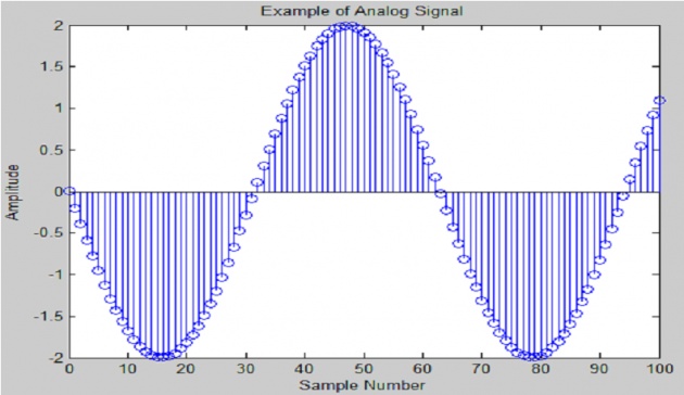
Digital signal is the one which can take countable finite values in range.
In MATLAB we can plot digital signal for example a random bipolar data using stem or plot
commands
%Digital Signal Example
d=round(rand(1,100)); %Random Values
bd=2*d-1; %binary data
phase=pi; %Phase
n=1:100; %Time axis
stem(n,bd);
title('Example of Digital Signal');
xlabel ('Time');
ylabel ('Amplitude');
Square wave is another example of Digital signal.
%Digital Signal Example
A=1; %Amplitude
f=2; %Frequence
phase=pi; %Phase
t=(0:0.01:2*pi)/pi; %Horizontal time axis
plot(t,A*square(2*pi*f*t+phase));
axis([-0.1,2.1,-1.1,1.1]);
title('Example of Digital Signal');
xlabel ('Time (pi Units)');
ylabel ('Amplitude');
3.3 Periodic vs. Aperiodic Signals:
a) Periodic Signals:
A signal which repeats its pattern after a specific interval of time is called periodic signal. A
signal which does not repeat its pattern after a specific interval of time is called aperiodic signal.
[ ] [ ]
Where N is the fundamental time period.
In MATLAB we can generate a periodic signal using following code:
%Periodic Signal Example
A=1; %Amplitude
f=1; %Frequence
phase=pi; %Phase
n=0:10; %Sample Number
stem(n,A*sin(f*n+phase));
title('Example of Periodic Signal');
xlabel ('n (Sample Number)');
ylabel ('Amplitude'); 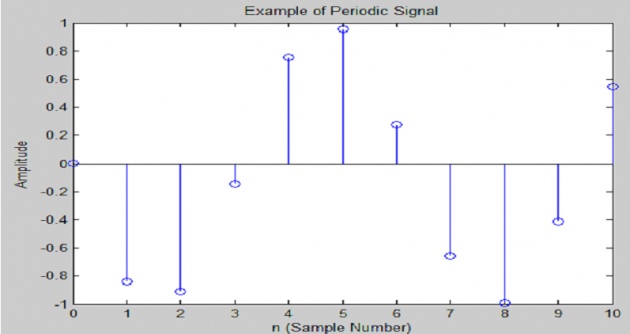
b) Aperiodic Signals:
The opposite of a periodic signal is an aperiodic signal. Aperiodic function never repeats,
although technically an aperiodic function can be considered like a periodic function with an
infinite period.
In MATLAB we can generate an Aperiodic signal using following code:
%Aperiodic Signal Example
A=1; %Amplitude
f=1; %Frequence
phase=pi; %Phase
n=0:10; %Sample Number
plot(n,A*exp(f*n+phase));
title('Example of Aperiodic Signal');
xlabel ('n (Sample Number)');
ylabel ('Amplitude');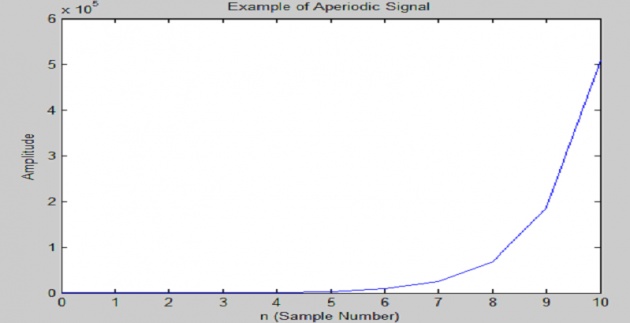
3.4 Even vs. Odd Signals
a) Even Signals:
If x(-n) = x(n) then signal is called even signal.
Cosine function is an example of even signal.
%Even Signal Example
A=1; %Amplitude
f=1; %Frequence
phase=pi; %Phase
n=0:10; %Sample Number
plot(n,A*cos(f*n+phase));
title('Example of Even Signal');
xlabel ('n (Sample Number)');
ylabel ('Amplitude');
b) Odd Signals:
If x(-n) = -x(n) then signal is called odd signal. Sine function is a n example of odd signal.
%Odd Signal Example
A=1; %Amplitude
f=1; %Frequence
phase=pi; %Phase
n=0:10; %Sample Number
plot(n,A*sin(f*n+phase));
title('Example of Odd Signal');
xlabel ('n (Sample Number)');
ylabel ('Amplitude');
3.5 Deterministic vs. Random Signals
a) Deterministic Signal:
A deterministic signal is one which can be completely represented by Mathematical equation at any time. In a deterministic signal there is no uncertainty with respect to its value at any time. All the examples given above are of deterministic signals.
b) Random Signal:
Stochastic signals, or random signals, are not so nice. Random signals cannot be characterized by a simple, well-defined mathematical equation and their future values cannot be predicted. Rather, we must use probability and statistics to analyze their behavior. Also, because of their randomness, average values from a collection of signals are usually studied rather than analyzing
one individual signal.
Example: Rolling a dice 1000 times.
one=0;two=0;three=0;four=0;five=0;six=0;%Possible Outcomes
a=ceil(6*rand(1,1000)); %1000 rolls of dice
for i=1:1000 %Counting each outcome
if(a(i)==1)
one=one+1;
end
if(a(i)==2)
two=two+1;
end
if(a(i)==3)
three=three+1;
end
if(a(i)==4)
four=four+1;
end
if(a(i)==5)
five=five+1;
end
if(a(i)==6)
six=six+1;
end
end
%Probability of each outcome
probDice(1)=one/1000;
probDice(2)=two/1000;
probDice(3)=three/1000;
probDice(4)=four/1000;
probDice(5)=five/1000;
probDice(6)=six/1000;
stem(probDice);%Plot each outcome
axis([0 7 0 0.25]);
xlabel('Numbers 1,2,3,4,5 and 6 on the Dice');
ylabel('Probability of 1,2,3,4,5 and 6 after 1000 experiments');
title('Probability of each number after roll of Dice 1000
times');
3.6 Energy vs. Power Signal:
a) Energy Signal:
A signal x(t) is said to be energy signal if and only if the total normalized energy is finite and
non-zero. Non-periodic signals are energy signals.
Total energy of a signal x(t) can be expressed as:
b) Power Signal:
The signal x(t) is said to be power signal, if and only if the normalized average power p is finite and non-zero. Practical periodic signals are power signals.
Total power of a signal x(t) is given by:
Example: Following is example of Energy signal:
Let {
| |
| |
Using MATLAB Symbolic Maths, we can find its energy as following
syms t T
x=2;
E=limit((int(x^2,t,-1,1)),T,inf)
E =
8
For an energy signal, power will always be equal to zero
P=limit((1/(2*T))*(int(x^2,t,-1,1)),T,inf)
P =
0
Example: Following is the example of Power Signal
Let {
syms t T
x = 2;
P = limit((1/(2*T))*(int(x^2,t,-T,T)),T,inf)
P =
4
For a power signal, energy is always equal to .
E = limit((int(x^2,t,-T,T)),T,inf)
E =
Inf
Example: Following is the example of a signal which is neither a power signal nor energy signal
for which we have Total energy and power equal to .
Let {
syms t T
x=t;
E=limit((int(x^2,t,-T,T)),T,inf)
E =
Inf
P=limit((1/(2*T))*(int(x^2,t,-T,T)),T,inf)
P =
Inf
Power and Energy of Discrete Time Signals
For a Discrete Time Signal we simply replace integral with summation. In MATLAB symsum
command is used for summation.
Example: Find the energy of the following signal.
[ ]
syms n T
E=limit((symsum(sin(n*pi)^2,n,-4,4)),T,inf)
E =
0
P=limit((1/(2*T))*(symsum(x^2,t,-T,T)),T,inf)
P =4